Natural Language Processing

以前一定要從語言學去分析，才能處理比較好。
現在都用統計的方式做，雖然人看不懂，但效果更好。

Information Retrieval (IR): 資訊檢索

Stemming: 詞幹還原
Lemmatization: 詞形還原
Stop Words: 常見但無意義的詞彙（如 “the”, “is”, “in”）
Term Frequency (TF): 詞彙在文件中出現的頻率
- $TF(t, d) = \frac{f_{t,d}}{\sum_{t’ \in d} f_{t’,d}}$
Inverse Document Frequency (IDF): 詞彙在整個語料庫中出現的稀有程度
- $IDF(t) = \log(\frac{N}{DF(t)})$
  - $N$: 文件總數
  - $DF(t)$: 包含詞彙 $t$ 的文件數
- 同個 Feature 如果所有文本都有出現，代表他沒甚麼重要性，所以越稀有的詞彙，IDF 越高越重要
Cosine Document Similarity: 衡量兩個向量之間的相似度
- $Cosine_Document_Similarity(A, B) = \frac{A \cdot B}{||A|| \times ||B||}$
BM25: 一種改進的 TF-IDF 權重計算方法，計算文件與查詢的相關性
- $BM25(t, d) = IDF(t) \times \frac{f_{t,d} \times (k_1 + 1)}{f_{t,d} + k_1 \times (1 - b + b \times \frac{|d|}{avgdl})}$
  - $k_1$ 和 $b$ 是調整參數
  - $|d|$: 文件長度
  - $avgdl$: 平均文件長度

Word Representation: 詞彙表示

Bag of Words (BoW): 將文本表示為詞彙的無序集合，忽略語法和詞序
One-hot Encoding: 將詞彙表示為高維稀疏向量，只有對應詞彙的位置為 1，其餘為 0
Word Embeddings (dense space): 將詞彙映射到低維連續向量空間，捕捉詞彙之間的語義關係
Latent Semantic Analysis (LSA): 使用奇異值分解 (SVD) 將詞彙和文件映射到潛在語義空間
Continuous Bag of Words (CBOW): 預測中心詞彙，給定上下文詞彙
Skip-gram: 預測上下文詞彙，給定中心詞
part of speech (POS): 分析詞性
word sense ambiguity (WSA): 詞義歧異
N-grams: 連續 n 個字詞的組合
- unigram: 1 個字詞
- bigram: 2 個字詞
- trigram: 3 個字詞
- 越長越短都有各自的優缺點
Linguistic Signature: 獨特且可辨識的語言模式
Perplexity (PPL): 衡量語言模型預測下一個字詞的困難程度
- $PPL(W) = P(w_1, w_2, …, w_N)^{-1/N}$
- PPL 越低，表示模型越好
- 在 Fine-tuning 的時候，可以用來評估模型是不是保有原有的語言能力
TF-IDF: 衡量詞彙在文件中的重要性
- $TF-IDF(t, d) = TF(t, d) \times IDF(t)$
PPMI (Positive Pointwise Mutual Information): 衡量詞彙與上下文之間的關聯強度
- $PMI(t, c) = \log(\frac{P(t, c)}{P(t) \times P(c)})$
- $PPMI(t, c) = \max(PMI(t, c), 0)$
  - $P(t, c)$: 詞彙 $t$ 和上下文 $c$ 同時出現的概率
  - $P(t)$: 詞彙 $t$ 出現的概率
  - $P(c)$: 上下文 $c$ 出現的概率
Word2Vec: 基於 nn 的詞嵌入方法，包括 CBOW 和 Skip-gram 兩種模型
- 要定義 Positive Sample 和 Negative Sample，且兩者比例要適當
Contextualized Embeddings: 根據上下文動態生成詞嵌入，想是 BERT、GPT
- 同一個詞彙在不同上下文中會有不同的表示，像是 bank 在 river bank 和 financial bank 中會有不同的向量
Name Entity Recognition (NER): 識別文本中的專有名詞，如人名、地名、組織名等

RNN

RNNs for NER
RNNs for Sequence Classification
Stacked RNNs
Bidirectional RNNs
- 結合前向和後向的 RNN，捕捉上下文資訊
Bidirectional RNNs for Sequence Classification

Sequence to Sequence Models

機器翻譯
文件摘要
對話生成
RNN for Sequence Generation
RNN for Machine Translation
- context vector
- RNN 需要 End to End 的訓練，做摘要和做翻譯訓練出來的 Decoder 不一樣

Long Short-Term Memory (LSTM)

大量的訓練參數，為了捨棄不重要的資訊，只保留重要的資訊。能稍為解決 Vanishing/ Exploding Gradient 的問題，但還是會有。

最大的問題是依然不能平行化

Forget Gate
Input Gate
Candidate MEmory
Output Gate

Attention Mechanism

讓模型能夠專注於輸入序列的特定部分，而不是像傳統 RNN 那樣一次處理整個 Sequence。

Attention with RNNs

一開始是把 Attention 接上 RNN ，把每個時間點的 Hidden State 都拿來算 Attention。但是這樣還是有 RNN 的缺點，無法平行化。

Attention without RNNs

Transformer 就是完全用 Attention 機制來取代 RNN，讓模型能夠平行化處理序列資料。

Sub-word Tokenization

Common Methods

Delimiter-based Segmentation: 以空格或標點符號作為分隔符來切詞
- 像英文這種拼音型的語言可以用空格切詞，但像中文、日文就沒辦法。
- 對於翻譯任務來說，不一定是 1 to 1 的對應關係。

基於上述問題，後來發展出一些統計上的方法：

Byte Pair Encoding (BPE)

基於頻率的子詞切分方法，將最常見的字元對合併成子詞單位

$$
\begin{aligned}
\text{Final Vocabulary Size} &= \text{Initial Vocabulary Size} + \text{Number of Merges}
\end{aligned}
$$

BPE 是基於 Greedy Algorithm，最高頻率的不一定是最好的選擇，像是 Hello World 會被切成 Hell + o + World，因為 Hell 本身也是一個詞彙。
不過其實也不會影響太大，BPE 已經很夠用，GPT 系列也是用這個。

Unigram Language Model

每個 subword 都有一個機率，演算法會選出能最大化整句機率的分割方式。

ELMo, BERT, GPT, and T5 (BERT and its Family)

Pretrained Word Embeddings 是靜態的，無法根據上下文改變詞彙的表示，像是 I record a record，兩個 record 的意思不一樣，但 Embedding 是一樣的，因此應該要能夠根據上下文改變詞彙的表示。

ELMo (Embeddings from Language Models)

Bidirectional Language Model (biLM)
- 使用雙向 LSTM 來捕捉詞彙的語義資訊，能根據上下文動態生成 word embeddings
生不逢時，ELMo 發表的時候，Transformer 已經出來了，且效果更好

Encoder-based Models: BERT

Bidirectional Encoder Representations from Transformers (BERT)

使用 Transformer 的 Encoder 結構，捕捉遠距離的依賴關係
Masked Language Model (MLM): 隨機遮蔽輸入序列中的部分詞彙，讓模型預測被遮蔽的詞彙 (克漏字)
Next Sentence Prediction (NSP): 預測兩個句子是否連續出現
- 後來發現這個任務沒什麼幫助，反而刪掉效果更好
直接訓練會太呆版，所以會加入一些隨機性
- 對於 Training Set 的 15% 的 Token 做 Mask
  - 80% 的機率換成 [MASK]
  - 10% 的機率換成隨機的 Token
  - 10% 的機率不變
訓練好的 BERT 可以用來做下游任務的 Fine-tuning
BERT 的輸入格式
- [CLS]：句子開始標記
- [SEP]：句子分隔標記
不同任務會有不同的輸出方式
- 分類任務：使用 [CLS] 的輸出向量 (情感分析)
- 序列標註任務：使用每個 Token 的輸出向量 (NER, POS)

Limitations of Encoders

無法做生成相關的任務 (如：QA、對話生成)

Encoder-Decoder Models: T5

Text-to-Text Transfer Transformer (T5)

使用 Transformer 的 Encoder-Decoder 結構
將所有 NLP 任務都轉換為文本到文本的格式
- 例如：情感分析任務，輸入為 “classify sentiment: I love this movie!”，輸出為 “positive”
靠著大量的資料讓模型硬學會各種任務

Extensions of T5: BART

Bidirectional and Auto-Regressive Transformers (BART)
Token Masking, Token Deletion, Text Infilling, Sentence Permutation, Document Rotation

Decoder-based Models: GPT

2018 年 OpenAI 發表 GPT，使用 Transformer 的 Decoder 結構，作者是 Alec Radford
一開始效果沒有很好，後來 GPT-2、GPT-3、GPT-4 效果越來越好
使用自回歸語言模型 (Auto-Regressive Language Model, ARLM)
- 根據前面的詞彙預測下一個詞彙

GPT-3

有 1750 億個參數
發現大型模型有 Emergent Abilities
- 隨著模型規模增大，會出現一些小模型沒有的能力

In-context Learning

不需要微調模型，只要在輸入中提供一些範例，模型就能學會任務
分為 Few-shot Learning、One-shot Learning、Zero-shot Learning
沒有實際跟新模型的參數

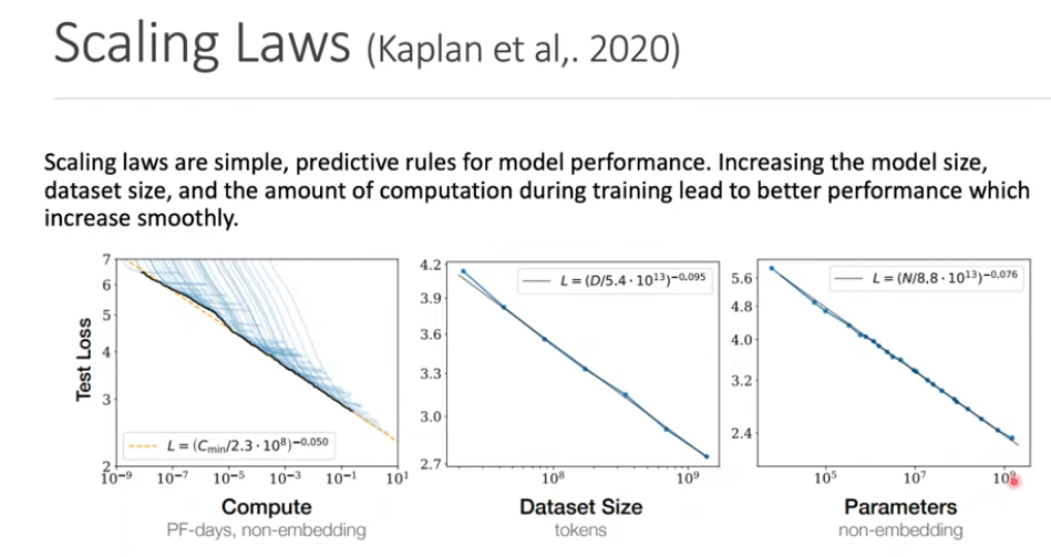
Scaling Laws

模型的性能與參數數量、訓練資料量和計算資源之間存在一定的關係

Decoding Strategies and Evaluation for Natural Language Generation

Natural Language Generation (NLG)

生成 text 的過程就叫做 NLG
- Machine Translation
- Abstractive Summarization
- Dialogue Generation (e.g., ChatGPT)
- Story Generation
- Image Captioning

How to Train a Conditional Language Model

如果是翻譯任務，會需要平行語料庫 (source, target)
Teacher Forcing: 在訓練過程中，使用真實的前一個詞彙作為輸入，而不是模型預測的詞彙
- 可以加速收斂，但會導致 Exposure Bias
- 不用的話通常結果很爛

Greedy Decoding

每次都選擇機率最高的詞彙作為輸出
- 優點：簡單且快速
- 缺點：容易陷入局部最優解，生成的文本可能缺乏多樣性
Top-K Sampling
- 在生成過程中，先選擇前 K 個機率最高的詞彙，然後從中進行隨機抽樣
- 有可能選到機率很低的詞彙，導致生成的文本不連貫
Nucleus Sampling (Top-p Sampling)
- 選擇累積機率達到 p 的詞彙集合，然後從中進行隨機抽樣
Beam Search
- 同時維護多個候選序列，選擇最有可能的序列作為最終輸出
- 但是越長的句子會被懲罰，機率會越來越小，所以需要做 Normalization

How to Evaluate NLG Models

BLEU (Bilingual Evaluation Understudy)

計算 n-gram 的 precision
- Unigrams -> BLEU-1
- Bigrams -> BLEU-2
- Trigrams -> BLEU-3
- 4-grams -> BLEU-4
Precision: 你猜的答案中有多少是對的
- $Precision = \frac{|\text{Relevant and Retrieved instances}|}{|\text{All Retrieved instances}|}$
Recall: 正確答案中有多少被你猜出來
- $Recall = \frac{|\text{Relevant and Retrieved instances}|}{|\text{All Relevant instances}|}$
Example:
- Chinese: 我想要讀那本書
- Reference1: I want to read that book
- Reference2: I want to read the book
- Model Output: the the the the the the
- Precision = 6/6 = 1
Brevity Penalty (BP): 懲罰過短的句子
因為分母是生成句子的長度，分子是參考句子的長度，如果生成的句子太短，precision 通常會比較高，但這樣不合理，所以要加上 BP 來懲罰過短的句子

$$
BP =
\begin{cases}
1 & \text{if } c > r \newline
e^{(1 - r/c)} & \text{if } c \leq r
\end{cases}
$$
- $c$: candidate translation length
- $r$: reference translation length
最終 BLEU 分數計算：

$$
BLEU = BP \cdot \exp\left( \sum_{n=1}^{N} w_n \log p_n \right)
$$
- $p_n$: n-gram precision
- $w_n$: n-gram 的權重，通常均等分配
- $N$: 最大 n-gram 長度

ROUGE (Recall-Oriented Understudy for Gisting Evaluation)

ROUGE-N: 計算 n-gram 的 recall

$$
ROUGE-N = \frac{\sum_{S \in \text{Reference Summaries}} \sum_{\text{gram}n \in S} \text{Count}{\text{match}}(\text{gram}n)}{\sum{S \in \text{Reference Summaries}} \sum_{\text{gram}_n \in S} \text{Count}(\text{gram}_n)}
$$
ROUGE-L: 計算兩個序列的 Longest Common Subsequence (LCS)

NLP Benchmarks

GLUE (General Language Understanding Evaluation)

總共有 9 個任務
任務可以分成三類
- Single-Sentence Tasks
  - 模型只需要理解單一句子的語義
  - CoLA (Corpus of Linguistic Acceptability): 判斷句子是否符合語法規則
  - SST-2 (Stanford Sentiment Treebank): 判斷句子的情感傾向（正面或負面）
- Sentence Pair Tasks
  - 模型需要理解兩個句子之間的關係
  - MNLI (Multi-Genre Natural Language Inference): 判斷兩個句子之間的邏輯關係（蕴涵、中立、矛盾）
  - RTE (Recognizing Textual Entailment): 判斷兩個句子是否存在蕴涵關係 (簡化版 MNLI)
  - QQP (Quora Question Pairs): 判斷兩個問題是否具有相同的語義
  - MRPC (Microsoft Research Paraphrase Corpus): 判斷兩個句子是否為同義句
  - QNLI (Question Natural Language Inference): 判斷問題和句子之間的蕴涵關係
- Semantic Similarity Tasks
  - STS-B (Semantic Textual Similarity Benchmark): 評估兩個句子之間的語義相似度，分數範圍為 0 到 5
最後分數會綜合各個任務的結果，不過有時候會只看部分任務的結果

SQuAD (Stanford Question Answering Dataset)

由 Stanford 大學釋出的閱讀理解資料集
SQuAD 1.1: 包含 100,000 個問題，答案都是文章中的一段文字
SQuAD 2.0: 在 SQuAD 1.1 的基礎上增加了無答案的問題，模型需要判斷問題是否有答案

MMLU (Massive Multitask Language Understanding)

包含 57 個不同領域的多選題
測試模型在各種專業知識領域的理解能力
涵蓋範圍廣泛，包括 STEM、Humanities、Social Sciences 等等
模型需要在沒有額外訓練的情況下，直接回答這些問題

MTEB (Massive Text Embedding Benchmark)

評估文本嵌入 (Text Embedding) 模型在多種任務上的表現
包含文本分類、文本生成、文本相似度等多個任務

Watermark for text

GPT-3, InstructGPT, and RLHF

GPT-1

Decoder-only Transformer
12 層，117M 個參數

GPT-1

GPT-2

Layer Normalization 放在每個 sub-block 的前面
最後的 self-attention layer 後面多加一個 Layer Normalization
GPT-2-medium: 24 層，345M 個參數
GPT-2-large: 36 層，762M 個參數
GPT-2-xl: 48 層，1.5B 個參數

GPT-2

GPT-3

Sparse Transformer
- 與其讓每個 token 都看所有 token，不如讓它只看「部分有意義的 token」。
- 大幅減少計算量，且效果不會差太多

Instruct Tuning

一種微調方法，讓模型能夠更好地理解和執行人類的指令
讓模型更理解人類語氣與意圖，提升泛化與實用性，可以回答沒有看過的問題。

InstructGPT (GPT-3.5)

InstructGPT 是在 GPT-3 的基礎上，透過 人類標註與反饋 進行再訓練

訓練過程是，先學人類怎麼說，再學人類喜歡怎麼說。

監督式微調 (Supervised Fine-tuning, SFT)

讓模型學會如何「遵循指令」

收集一個由人類標註者撰寫的高品質「指令-回應」資料集。使用這個資料集來微調 (fine-tuning) 一個預訓練好的基礎模型 (如 GPT-3)。

產生 SFT 模型。這個模型能理解並執行指令，但回答的品質可能還不夠穩定或不符合人類偏好。

訓練獎勵模型 (Reward Model, RM)

訓練一個模型來 「評估回應的品質」，使其學會人類的偏好。

使用上一步的 SFT 模型，針對一個指令（prompt）產生多個不同的回應。人類標註者排序 (ranking) 這些回應（例如：從最好到最差）。使用這些「排序資料」來訓練一個新的模型，即獎勵模型 (RM)。

產生 RM。這個模型會為任何「指令-回應」組合打一個分數 (reward)，分數越高代表越符合人類偏好。

使用強化學習 (Reinforcement Learning)

利用 RM 作為「評審」，進一步優化 SFT 模型，使其產生的回應能獲得最高的「獎勵分數」。

將 SFT 模型（在 RL 術語中稱為「策略 Policy」）複製一份。讓 Policy 針對新的指令產生回應。讓獎勵模型 (RM) 為這個「指令-回應」組合打分 (reward)。使用這個 reward 分數，透過 RL 演算法 (PPO, Proximal Policy Optimization) 來更新 Policy 模型的參數。

產生最終的 InstructGPT 模型。這個模型被訓練成傾向於產生那些「RM 會給高分」的回應，而 RM 的評分標準又來自於人類的偏好。

HW3: Multi-output learning

標點符號轉換

把中文標點符號轉換成英文標點符號

token_replacement = [
    ["：" , ":"],
    ["，" , ","],
    ["“" , "\""],
    ["”" , "\""],
    ["？" , "?"],
    ["……" , "..."],
    ["！" , "!"]
]

載入 BERT tokenizer

bert-base-uncased 是 Google 原版 BERT 模型的一個預訓練版本名稱，只用小寫字母，不區分大小寫。

1	`tokenizer = BertTokenizer.from_pretrained("google-bert/bert-base-uncased", cache_dir="./cache/")`

建立 SemevalDataset 類別

一個自訂的 Dataset 類別，告訴 PyTorch 怎麼讀取資料。

init：用 load_dataset 從 Hugging Face 下載 sem_eval_2014_task_1 資料集，並指定要載入 train、validation 還是 test 部分。
len：讓 PyTorch 知道這個資料集總共有多少筆資料。
getitem：當 DataLoader 需要資料時，它會呼叫這個函式。它會取得第 index 筆資料，對 premise 和 hypothesis 進行標點替換，然後回傳這個處理過的字典。

class SemevalDataset(Dataset):
    def __init__(self, split="train") -> None:
        super().__init__()
        assert split in ["train", "validation", "test"]
        self.data = load_dataset(
            "sem_eval_2014_task_1",
            split=split,  # 只載入指定的資料集部分
            trust_remote_code=True,  # 允許執行該資料集 repo 裡的自定義程式碼
            cache_dir="./cache/"  # 指定快取目錄
        ).to_list()

    def __getitem__(self, index):
        d = self.data[index]
        # Replace Chinese punctuations with English ones
        for k in ["premise", "hypothesis"]:
            for tok in token_replacement:
                d[k] = d[k].replace(tok[0], tok[1])
        return d

    def __len__(self):
        return len(self.data)

資料 batch 處理函式

DataLoader 會一次抓好幾筆資料 (batch_size)，然後把這些資料丟給 collate_fn 來打包。

tokenizer(...)：
它會把 premise 和 hypothesis 兩個句子打包成 BERT 喜歡的格式：[CLS] 句子 A [SEP] 句子 B [SEP]。
- padding=True：把這 8 筆資料補到一樣長。
- truncation=True：句子太長就咖掉。
- return_tensors=”pt”：轉成 PyTorch Tensors。
打包標籤 (Labels)：
- 程式會先檢查一下 (if … in …)，看看這批資料有沒有 relatedness_score 和 entailment_judgment 這兩個答案。
- 如果有 (像 train 和 validation 資料集)，就把它們收集起來轉成 Tensors。
- 如果沒有 (像 test 資料集)，那就回傳 None (代表「沒答案」)。
- return：回傳一個字典，裡面有模型要吃的 inputs 和 labels。

def collate_fn(batch):
    premises = [d['premise'] for d in batch]
    hypotheses = [d['hypothesis'] for d in batch]

    # Tokenize the sentence pairs
    inputs = tokenizer(
        premises,
        hypotheses,
        padding=True, # 對齊到本 batch 中最長序列（動態 padding）
        truncation=True, # 若超過 max_length 會截斷
        return_tensors="pt", # 讓輸出直接是 PyTorch tensors
        max_length=512 # 序列最長 512 token
    )

    # 取出語義相似度分數（連續值，迴歸任務）組成 FloatTensor
    relatedness_score = torch.tensor([d['relatedness_score'] for d in batch], dtype=torch.float)
    # 取出蘊含關係標籤（分類任務）組成 LongTensor
    entailment_judgment = torch.tensor([d['entailment_judgment'] for d in batch], dtype=torch.long)

    return {
        "inputs": inputs,
        "relatedness_score": relatedness_score,
        "entailment_judgment": entailment_judgment
    }

載入資料集和 DataLoader

ds_train = SemevalDataset(split="train")
ds_validation = SemevalDataset(split="validation")
ds_test = SemevalDataset(split="test")

dl_train = DataLoader(ds_train, batch_size=train_batch_size, shuffle=True, collate_fn=collate_fn)
dl_validation = DataLoader(ds_validation, batch_size=validation_batch_size, shuffle=False, collate_fn=collate_fn)
dl_test = DataLoader(ds_test, batch_size=validation_batch_size, shuffle=False, collate_fn=collate_fn)

建立多輸出模型

__init__：
- self.bert：去 Hugging Face 把預訓練好的 BERT 模型載下來。
- self.classification_head：蓋一個簡單的線性層，專門負責「分類」任務。
- self.regression_head：蓋另一個線性層，專門負責「迴歸」任務。
forward：
1. kwargs 會是 tokenizer 產生的輸入字典（input_ids, attention_mask, token_type_ids），直接解包丟進 BERT。
2. BERT 吐出 pooler_output，一份丟給分類頭、一份丟給迴歸頭。
3. 最後把兩個頭算出來的答案 (classification_logits 和 regression_output) 一起回傳出去。

# TODO2: Construct your model
class MultiLabelModel(torch.nn.Module):
    def __init__(self, *args, **kwargs):
        super().__init__(*args, **kwargs)
        # Load the base BERT model
        self.bert = BertModel.from_pretrained("google-bert/bert-base-uncased", cache_dir="./cache/")

        # BERT base hidden size is 768
        bert_hidden_size = self.bert.config.hidden_size

        # We will use the [CLS] token output (pooler_output) for both tasks
        # 1. A regression head for similarity (output 1 value)
        self.regression_head = torch.nn.Linear(bert_hidden_size, 1)

        # 2. A classification head for entailment (output 3 values for 3 classes)
        self.classification_head = torch.nn.Linear(bert_hidden_size, 3)

        # Dropout for regularization
        self.dropout = torch.nn.Dropout(0.1)

    def forward(self, **kwargs):
        # Write your code here
        # Forward pass
        # kwargs will contain input_ids, token_type_ids, attention_mask
        outputs = self.bert(**kwargs)

        # Get the pooler_output, which is the [CLS] token's representation
        # passed through a Linear layer and Tanh activation. Shape: (batch_size, 768)
        # 專門給句子分類用的 pooled 向量（來自 [CLS] token 經線性層與 tanh
        cls_output = outputs.pooler_output
        cls_output = self.dropout(cls_output)

        # Pass the [CLS] output to both heads
        # (batch_size, 3)
        classification_logits = self.classification_head(cls_output)

        # (batch_size, 1)
        regression_output = self.regression_head(cls_output)

        return classification_logits, regression_output

設定模型、優化器、損失函數和評分工具

model = MultiLabelModel().to(device)
optimizer = AdamW(model.parameters(), lr=lr)

# 分類用的損失函數 (CrossEntropy)
loss_fn_classification = torch.nn.CrossEntropyLoss()
# 迴歸用的損失函數 (MSE，均方誤差)
loss_fn_regression = torch.nn.MSELoss()

# 載入評分工具
psr = load("pearsonr")
acc = load("accuracy")
best_score = 0.0

訓練與評估

import os

best_score = 0.0
os.makedirs('./saved_models', exist_ok=True)

for ep in range(epochs):
    pbar = tqdm(dl_train)
    pbar.set_description(f"Training epoch [{ep+1}/{epochs}]")
    model.train()

    total_train_loss = 0.0

    # TODO4: Write the training loop
    for batch in pbar:
        # Move data to device
        inputs = batch["inputs"].to(device)
        relatedness_score = batch["relatedness_score"].to(device)
        entailment_judgment = batch["entailment_judgment"].to(device)

        # clear gradient
        optimizer.zero_grad()

        # forward pass
        classification_logits, regression_output = model(**inputs)

        # compute loss
        # Squeeze regression output from (batch_size, 1) to (batch_size) to match labels
        loss_reg = loss_fn_regression(regression_output.squeeze(), relatedness_score)
        loss_class = loss_fn_classification(classification_logits, entailment_judgment)

        # Combine losses (simple addition)
        total_loss = loss_reg + loss_class

        # back-propagation
        total_loss.backward()

        # model optimization
        optimizer.step()

        total_train_loss += total_loss.item()
        pbar.set_postfix({"loss": total_loss.item()})

    print(f"Epoch {ep+1} Average Training Loss: {total_train_loss / len(dl_train)}")

    pbar = tqdm(dl_validation)
    pbar.set_description(f"Validation epoch [{ep+1}/{epochs}]")
    model.eval()

    all_sim_preds = []
    all_sim_labels = []
    all_ent_preds = []
    all_ent_labels = []

    # TODO5: Write the evaluation loop
    with torch.no_grad():
        for batch in pbar:
            # Move data to device
            inputs = batch["inputs"].to(device)
            relatedness_score = batch["relatedness_score"].to(device)
            entailment_judgment = batch["entailment_judgment"].to(device)

            # forward pass
            classification_logits, regression_output = model(**inputs)

            # Get predictions
            # Similarity predictions (regression)
            sim_preds = regression_output.squeeze().cpu().numpy()

            # Entailment predictions (classification)
            ent_preds = torch.argmax(classification_logits, dim=-1).cpu().numpy()

            # Collect all predictions and labels
            all_sim_preds.extend(sim_preds)
            all_sim_labels.extend(relatedness_score.cpu().numpy())
            all_ent_preds.extend(ent_preds)
            all_ent_labels.extend(entailment_judgment.cpu().numpy())

    # Compute metrics
    pearson_corr = psr.compute(predictions=all_sim_preds, references=all_sim_labels)['pearsonr']
    accuracy = acc.compute(predictions=all_ent_preds, references=all_ent_labels)['accuracy']

    print(f"Validation PearsonCorr: {pearson_corr:.4f}, Accuracy: {accuracy:.4f}")

    current_score = pearson_corr + accuracy
    if current_score > best_score:
        print(f"New best score ({current_score:.4f})! Saving model...")
        best_score = current_score
        torch.save(model.state_dict(), f'./saved_models/best_model.ckpt')

測試

# Load the model
model = MultiLabelModel().to(device)
model.load_state_dict(torch.load(f"./saved_models/best_model.ckpt", weights_only=True))

# Test Loop
pbar = tqdm(dl_test, desc="Test")
model.eval()

# Reset lists for test evaluation
all_sim_preds = []
all_sim_labels = []
all_ent_preds = []
all_ent_labels = []

with torch.no_grad():
    for batch in pbar:
        # Move data to device
        inputs = batch["inputs"].to(device)
        relatedness_score = batch["relatedness_score"].to(device)
        entailment_judgment = batch["entailment_judgment"].to(device)

        # forward pass
        classification_logits, regression_output = model(**inputs)

        # Get predictions
        sim_preds = regression_output.squeeze().cpu().numpy()
        ent_preds = torch.argmax(classification_logits, dim=-1).cpu().numpy()

        # Collect all predictions and labels
        all_sim_preds.extend(sim_preds)
        all_sim_labels.extend(relatedness_score.cpu().numpy())
        all_ent_preds.extend(ent_preds)
        all_ent_labels.extend(entailment_judgment.cpu().numpy())

# Compute final test metrics
test_pearson_corr = psr.compute(predictions=all_sim_preds, references=all_sim_labels)['pearsonr']
test_accuracy = acc.compute(predictions=all_ent_preds, references=all_ent_labels)['accuracy']

#ai #machine learning #nlp

Natural Language Processing

https://933yee.github.io/notes/2025/09/24/nlp/

Author

Kevin Lee

Posted on

September 24, 2025

Licensed under

TOEIC Previous

數學筆記 Next